I’ve seen a few TF discussions about tickers that follow SPY closely but have cheaper options for smaller accounts. I think this is useful information so I’ve decided to compile some that I know. If you just want to see the tickers, I’ll put them in the comments below this post.
Please do your own research before trading these, many will be leveraged.
I’ve written some python code for a few metrics that I thought might be useful when comparing tickers. The code is here. I have no formal coding education so I apologise for the formatting. There is also a slim (read: very high) possibility that there are mistakes. I’m pretty sure the correlation coefficient , calculated beta and volume coefficient are accurate though, and they are the most useful.
All metrics (except for volume coefficient) are calculated using monthly adjusted close data from the past 5 years (60 months) sourced from yahoo finance.
Correlation coefficient is a measure of how correlated the ticker is against a benchmark (SPY in this case but you can change that if you copy the code). A value of 1.0 means that the two tickers are perfectly correlated, a value of -1.0 means that the tickers have a perfect negative correlation (inverse), and a value of 0 means there is no linear correlation.
Calculated Beta is a measure of the ticker’s volatility against a benchmark, a beta near 1.0 indicates that the ticker does not deviate from the benchmark, a beta <1 indicates that the ticker is less volatile than the benchmarch, and a beta >1 indicates that the ticker is more volatile than the benchmark. I’ve called this calculated beta as it differs from the beta data on yahoo finance.
Volume coefficient is just the average daily volume over the last month of the ticker divided by the average daily volume of the benchmark. A value of 2 means that the ticker experiences 2x as much average daily volume, a value of 0.5 means that the ticker experiences 0.5x as much daily volume. This is important as it will affect the bid-ask spread.
[size=4]I dont find these next metrics particularly useful for this but I made them anyway - you can skip to the comments[/size]
Novel-alpha is a measure of how well the ticker performs relative to the benchmark ticker. A novel-alpha of 1.2 means that the ticker has performed 1.2x better in percentage gain, a reading of 0.8 means that the ticker performed 0.8x as well etc. I’ve named it novel-alpha so it’s not confused with alpha (α) but it does describe a similar thing.
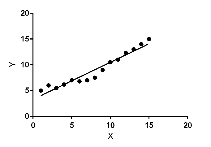
Novel-gamma is made to be used with novel-alpha. The percentage price increase is plotted against time and the regression line is calculated (line of best fit). The gradient of the regression line for the benchmark is then subtracted from the gradient of the regression line for the ticker, this value then has +1 added so that it centres around 1.0 and not 0.0 to match the other metrics. This can be used in conjunction with novel-alpha to paint a clearer picture of price action. Example below.
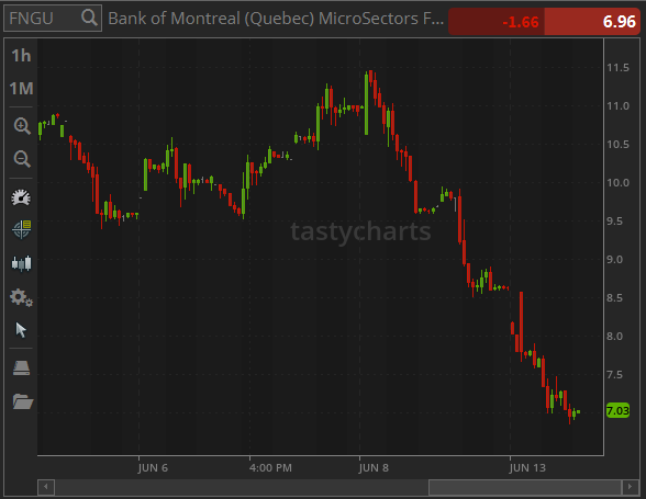
Graph 1:
Graph 2:
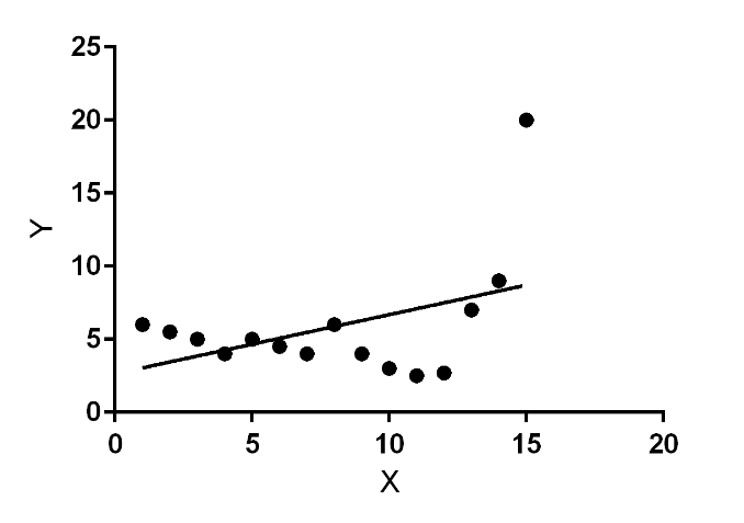
If you were to just use the novel-alpha values then it would appear that Graph 2 has had better performance but this misses important information. A novel-gamma below 1.0 indicates that there was a sudden rise in the stock price (graph 2), a value above 1.0 indicates that there was a sudden fall in stock price. Remember, this is all in relation to the benchmark, if novel-alpha is not close to 1.0 then you should disregard this interpretation of novel-gamma.
[center]
[/center]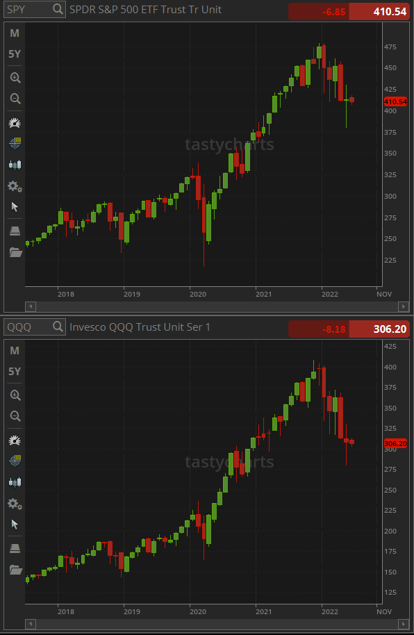
[center]
 [/center]
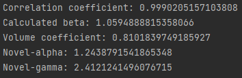
Above are the non-rounded values for QQQ using SPY as the benchmark. You can see that novel-alpha suggests that QQQ performed better than SPY but the novel-gamma is above 1.0 which indicates a steep climb and large drop. I believe this is because QQQ’s 52-week range experienced a 31.4% change and SPY’s experienced a 20.7% change.
[center]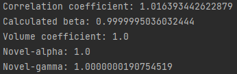 [/center]
Above are the non-rounded values when SPY is compared against itself. The correlation coefficient has a slight inaccuracy but I believe this is due to the magnitude of precision in the way that NumPy calculates covariance (I don’t think this issue is large enough to warrant a new calculation using something other than NumPy). The rest of the values are slightly swayed just because of how floating-point numbers work.
Ideal alternatives should have these values as close to 1.0 as possible. I believe this is theoretically impossible because a cheaper price and high correlation would require a higher beta (I think ![]() ) , so there will always be a trade-off. I would say this means that you will always have to assume higher volatility for cheaper prices.
) , so there will always be a trade-off. I would say this means that you will always have to assume higher volatility for cheaper prices.
 [/center]
 [/center]
 [/center]
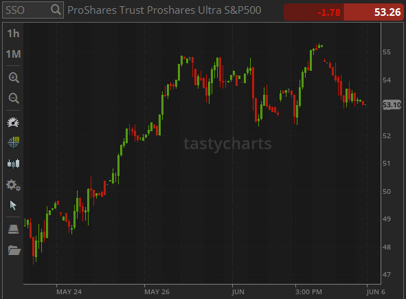 [/center]
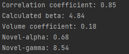
 [/center]
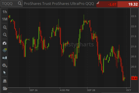 [/center]